First, install cmake, git and some additional packages. Under Ubuntu or Debian simply

sudo apt-get install cmake git build-essential libboost-all-dev

on any other platform you will need to install a C++ compiler a few libraries and the programs git and cmake. Now download and compile Auryn with the following commands

git clone https://github.com/fzenke/auryn.git
cd auryn/build/release
./bootstrap.sh && make

This will checkout the master branch and compile it in the subdirectory auryn/build/. At this point cmake will complain about any missing libraries. The static library libauryn.a will be placed under build/release/src/. I usually leave it there and tell my compiler explicitly where to find it, but you can also install it to your systems default directory using make install. For more detailed instructions on where to download and how to compile go to howto compile Auryn.

Now, let's run a first small Auryn simulation from the example directory

zenke@possum:~$ cd auryn/build/release/examples
zenke@possum:~/auryn/build/release/examples$
zenke@possum:~/auryn/build/release/examples$ ./sim_poisson 
[=========================] 100%      t=1.0s  f=5.2 Hz in SpikingGroup   
( 0) Freeing ...

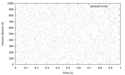
This will only take a few milliseconds and generate a bunch of Poisson spikes and store them in 'poisson.0.ras'. If you have gnuplot installed (sudo apt-get install gnuplot) you can visualize them from the command line with

echo "plot 'poisson.0.ras' with dots lc rgb 'black'" | gnuplot -p

For more details on this example go here.

Okay nice, let's do the same again for an actual network. Let's run a small balanced net, the Vogels Abbott benchmark net.

zenke@possum:~/auryn/build/release/examples$ ./sim_coba_benchmark --dir .
( 0) Setting up neuron groups ...
( 0) Setting up E connections ...
( 0) Setting up I connections ...
(!!) on rank 0: Use --fast option to turn off IO for benchmarking!
( 0) Setting up monitors ...
( 0) Simulating ...
[=========================] 100%      t=20.0s  f=17.5 Hz in NeuronGroup   
( 0) Saving elapsed time ...
( 0) Freeing ...

That should have been quick. Now let's look at what the network did. The simulation writes the spiking activity into files with the extension ras.

zenke@possum:~/auryn/build/release/examples$ ls -ltrs | tail -n 4
    8 -rw-rw-r--  1 zenke zenke     5776 Aug 18 10:30 sim_coba_benchmark.0.log
    4 -rw-rw-r--  1 zenke zenke        2 Aug 18 10:30 elapsed.dat
 3728 -rw-rw-r--  1 zenke zenke  3815326 Aug 18 10:30 coba.0.i.ras
15536 -rw-rw-r--  1 zenke zenke 15905529 Aug 18 10:30 coba.0.e.ras
zenke@possum:~/auryn/build/release/examples$ gnuplot 

	G N U P L O T
	Version 5.0 patchlevel 1    last modified 2015-06-07 

	Copyright (C) 1986-1993, 1998, 2004, 2007-2015
	Thomas Williams, Colin Kelley and many others

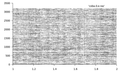
gnuplot> plot [1:2] 'coba.0.e.ras' with dots lc -1

which will plot the spikes of the excitatory cells between second 1 and 2:

Often your simulations will be slow to run, which is when it becomes important to run them using multiple CPUs or even multiple computers. Now let's run the same network as above using four CPUs in parallel:

zenke@possum:~/auryn/build/release/examples$ mpirun -n 4 ./sim_coba_benchmark --dir .
( 0) Setting up neuron groups ...
( 0) Setting up E connections ...
( 0) Setting up I connections ...
(!!) on rank 1: Use --fast option to turn off IO for benchmarking!
(!!) on rank 0: Use --fast option to turn off IO for benchmarking!
( 0) Setting up monitors ...
( 0) Simulating ...
(!!) on rank 3: Use --fast option to turn off IO for benchmarking!
(!!) on rank 2: Use --fast option to turn off IO for benchmarking!
[=========================] 100%      t=20.0s  f=17.0 Hz in NeuronGroup   
( 0) Saving elapsed time ...
( 0) Freeing ...
zenke@possum:~/auryn/build/release/examples$ ls -ltrs | tail -n 8
 876 -rw-rw-r--  1 zenke zenke  895414 Aug 18 10:31 coba.3.i.ras
3704 -rw-rw-r--  1 zenke zenke 3789934 Aug 18 10:31 coba.3.e.ras
 944 -rw-rw-r--  1 zenke zenke  965640 Aug 18 10:31 coba.2.i.ras
3648 -rw-rw-r--  1 zenke zenke 3732223 Aug 18 10:31 coba.2.e.ras
 884 -rw-rw-r--  1 zenke zenke  904769 Aug 18 10:31 coba.1.i.ras
3680 -rw-rw-r--  1 zenke zenke 3767219 Aug 18 10:31 coba.1.e.ras
 912 -rw-rw-r--  1 zenke zenke  933733 Aug 18 10:31 coba.0.i.ras
3796 -rw-rw-r--  1 zenke zenke 3886227 Aug 18 10:31 coba.0.e.ras

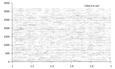
You just ran your first parallel simulation. As you can see this has generated more output files. If you plot the same one as before, you will seee something like this: there are fewer spikes. In fact, there are about one quarter of the spikes as compared to the plot above. The reason is that each CPU simulates a fraction of all the neurons and writes their spikes to independent output files. This way the simulation can run on physically different computers and the files can be written to independent disks. However, for your analysis you might want to merge them, which can be done easily on the Linux command line with the sort command

zenke@possum:~/auryn/build/release/examples$ sort -g -m coba.*.e.ras > coba_e_merged.ras

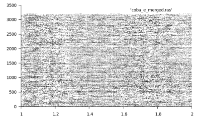
Plotting the spikes in coba_e_merged.ras yields: which should look similar to the network that was simulated using only a single CPU. In this case it won't look the same, because we used a different random seed for the connectivity matrix every time.

After you have compiled Auryn, you will probably want to familiarize yourself with the simulator using the supplied tutorials and examples. More on how to compile your own simulations here.